Extracting trends (VI) and national synthesis update

This post follows on from my previous posts on trend surface modelling (I)(II)(III)(IV)(V) and my posts on synthesis of multiple datasets using grid squares (I)(II)(III)(IV).

As our HER dataset is now nearly complete (only Merseyside is expected from now on; North Somerset and Bath & North East Somerset are unable to provide data), we are finally able to begin attempting to study the data which we have gathered on a nationwide scale.  Broad period classifications (Prehistoric; Bronze Age; Iron Age; Roman; early medieval; uncertain; “bad date” [i.e. outside our period]) were calculated for the HER data using a script (based upon the multitude of period designations applied by individual HERs or upon start / end dates) and the data was converted to shapefile format and merged into a single point layer.  This shapefile layer can then be very coarsely queried to produce distributions of records of different periods.

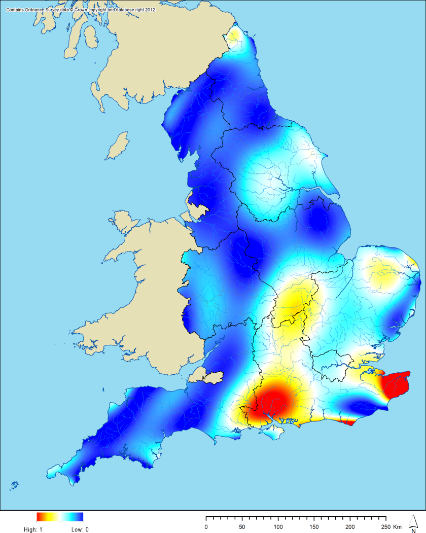
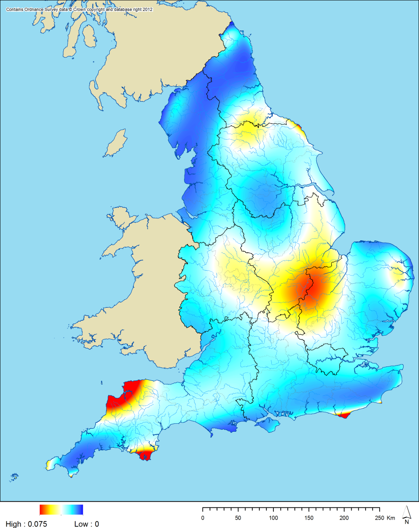
As an initial method for investigating this mass of data (around 400,000 records), I experimented with the production of a few trend surfaces.  First, one for all of the data received:
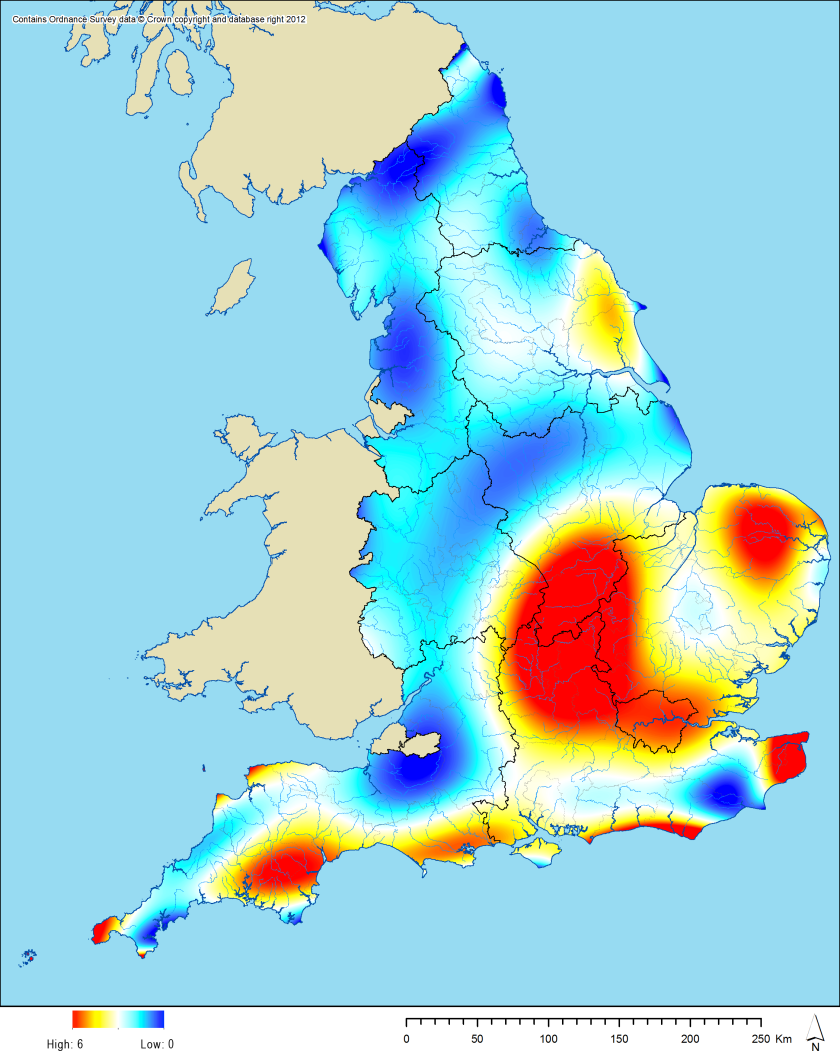
Trend surface for all EngLaId HER data

I think that there are two major factors at play in this trend.  The first is the general bias in English archaeology towards greater density of (probably) settlement and (certainly) fieldwork in the south and east of the country.  The second (possibly more dominant?) is the variation in recording methods used across the country.  Even where the same software is used, different HERs catalogue their data somewhat differently: some like to split everything up into individual periods and types, others like to collate into multi-period sites; some cast their nets wide to include as much data as possible (e.g. PAS data, MORPH data), others like to only include sites of certain and clear provenance.  This means that the density of data across the country is as much about modern practice as it is about activity in the ancient past.

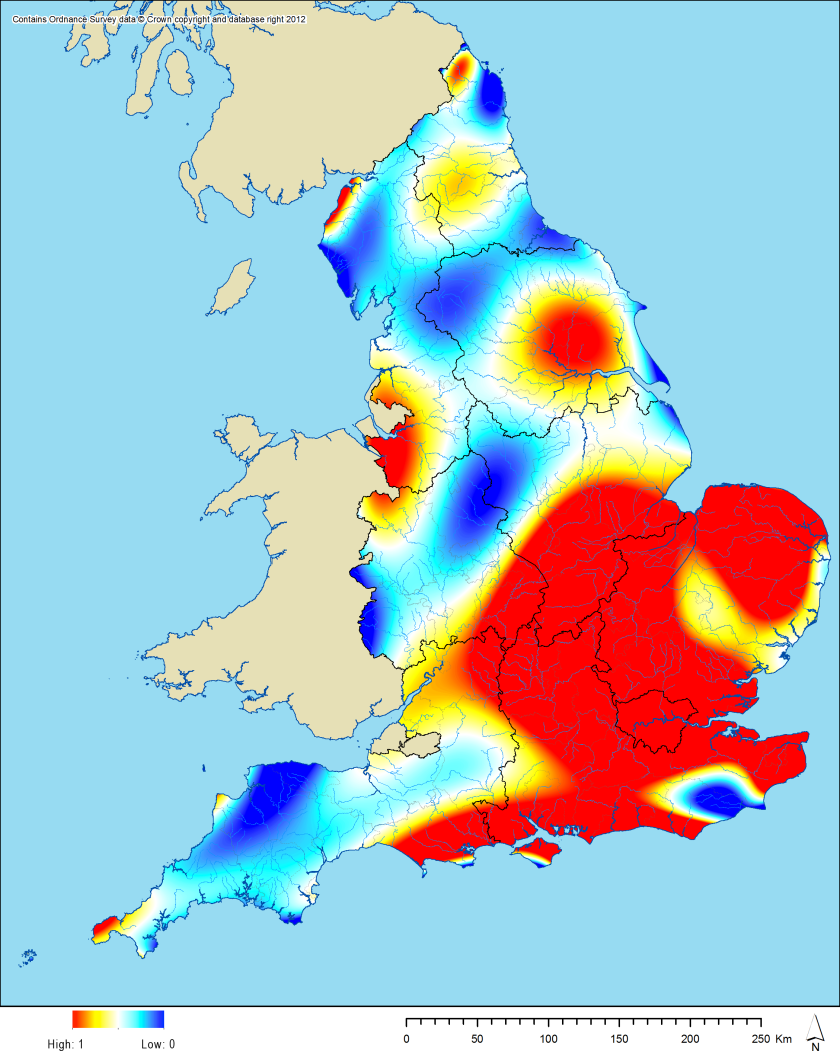
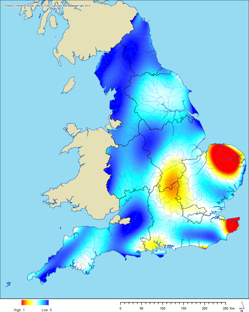
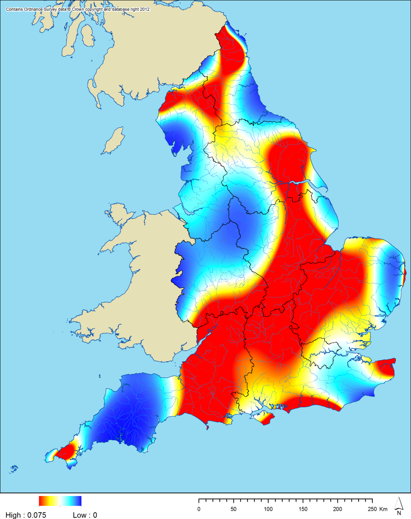
We can then produce similar surfaces for our broad periods (all to the same numerical scale):
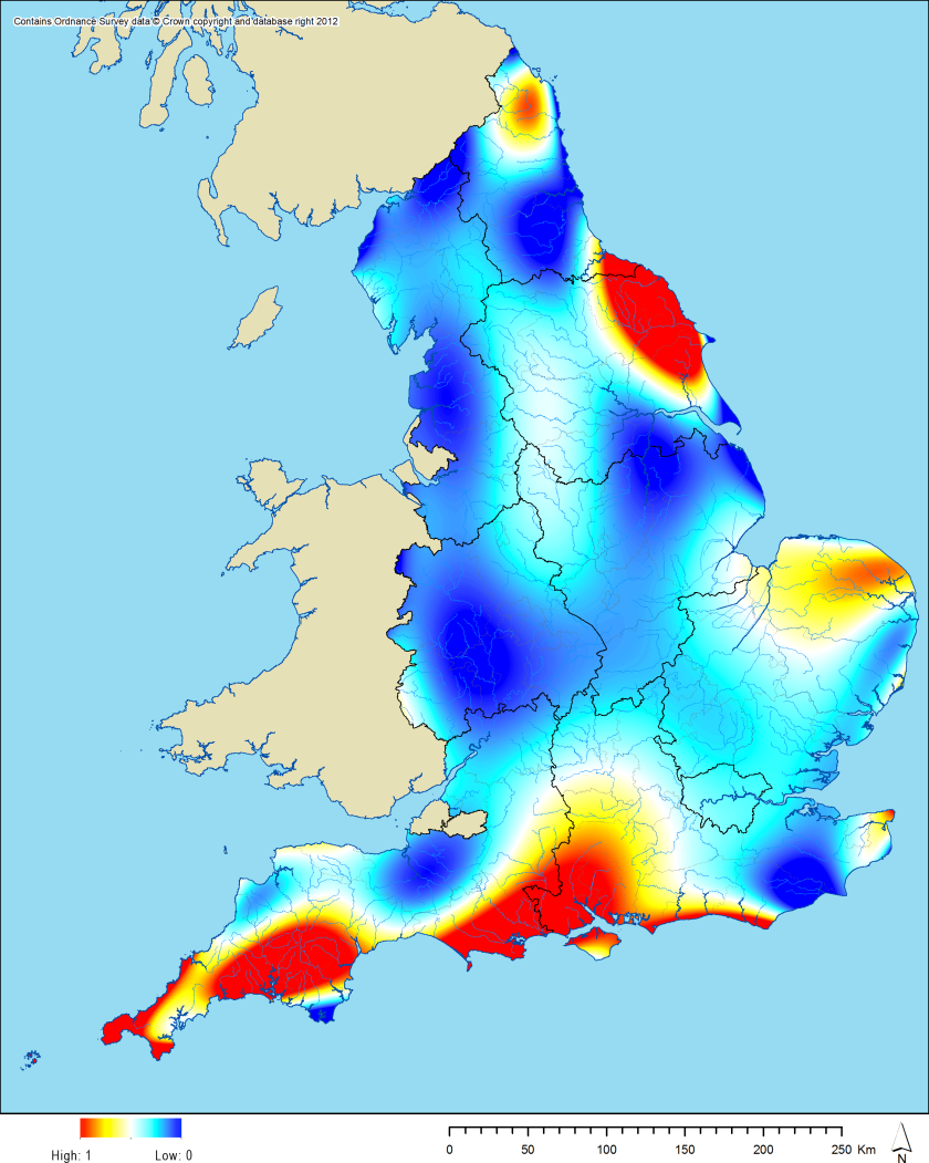
Trend surface for Bronze Age HER data
Trend surface for Iron Age HER data
Trend surface for Roman HER data
Trend surface for early medieval HER data

These four surfaces still reflect to some extent the differences seen in modern practice, but they are closer to the genuine distribution of past activity.  The Bronze Age surface seems to be biased towards uplands and towards Wessex.  The Iron Age surface has a clear bias towards the south east.  The Roman surface is biased towards lowland Britain but also towards the pockets of military activity in the north of England.  The early medieval surface is biased towards the eastern parts of England.

However, the distributions behind all of these trends are still heavily influenced by modern archaeological and CRM practices.  This is only going to get worse when we begin to produce duplication in our dataset by building in English Heritage NRHE data and other datasets.  As discussed in previous posts, one way in which to minimise these modern effects and reduce the influence of duplication is to collate data by 1 by 1 km grid cells.  This requires the application of a thesaurus containing simplified monument terms and the step already undertaken of assigning standardised period terms.  The result is a tessellation of 1 x 1 km grid squares across England recording the presence of different types of archaeological site for each of our broad periods, which we can then query and use to produce maps.

As an example, I constructed a few more trend surfaces, based upon the presence / absence of evidence for sites within our broad “domestic and civil” category.  This category includes: town, burh, civitas capital, colonia, hamlet, village, vicus, canabae legionis, oppidum, hillfort, anything defined using the word “settlement”, midden, timber platform (several of these sub-types belong to more than one broad category).  We can then look at how the underlying trends behind this category changed over time (these trend surfaces are logistic rather than linear, reflecting the probability of binary presence / absence relationship rather than density):
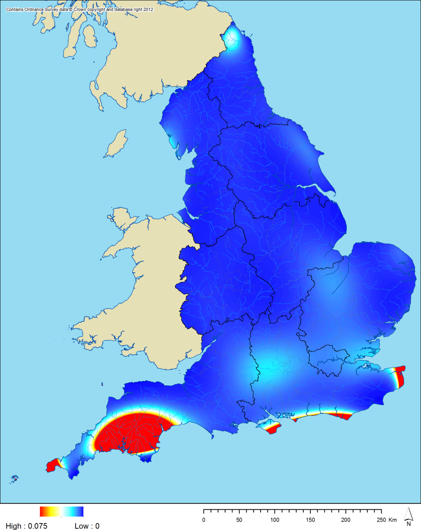
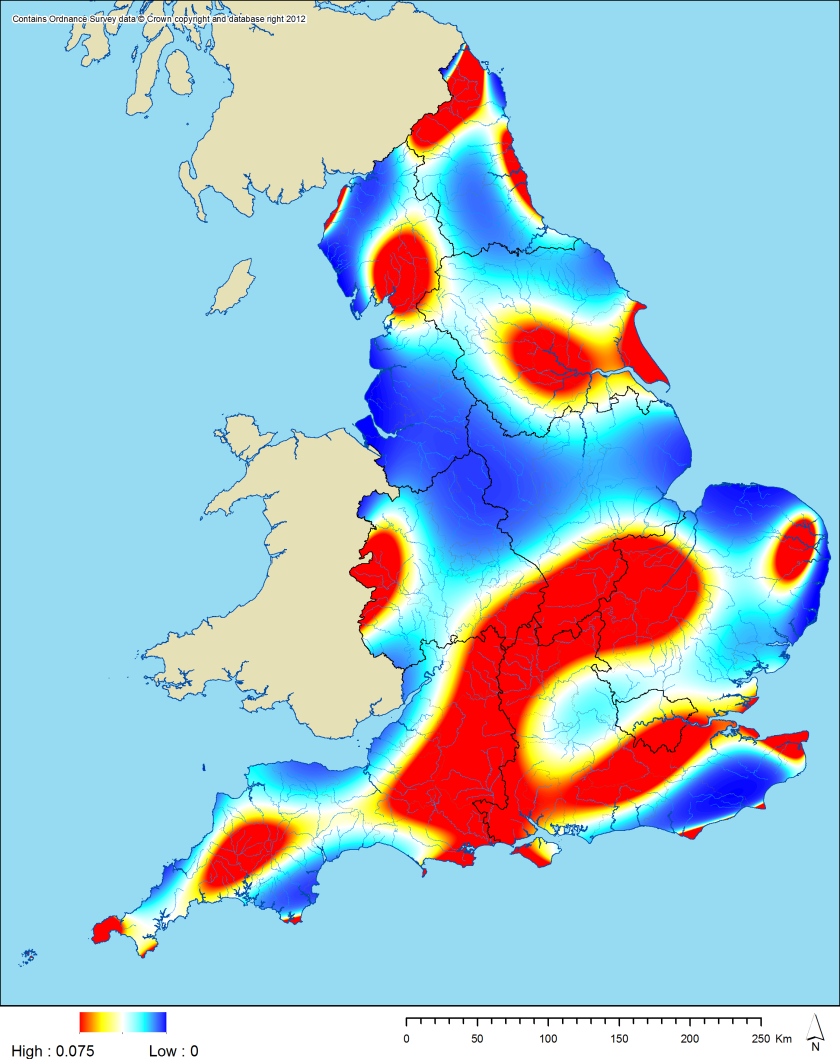
Trend surface (logistic) for synthesised data: Bronze Age "domestic and civil" category.
Trend surface (logistic) for synthesised data: Bronze Age “domestic and civil” category.
Trend surface (logistic) for synthesised data: Iron Age "domestic and civil" category.
Trend surface (logistic) for synthesised data: Iron Age “domestic and civil” category.
Trend surface (logistic) for synthesised data: Roman "domestic and civil" category.
Trend surface (logistic) for synthesised data: Roman “domestic and civil” category.
Trend surface (logistic) for synthesised data: early medieval "domestic and civil" category.
Trend surface (logistic) for synthesised data: early medieval “domestic and civil” category.

There is still some bias in these trend surfaces from the amount of data recorded by different modern archaeological entities (e.g. Northamptonshire is a very “completist” HER, which partially accounts for it showing up so strongly in many of the trend surfaces seen in this blog post), but the patterns are still quite interesting.  The Bronze Age is heavily influenced by the very high number of records present on Dartmoor and Bodmin Moor.  The Iron Age is probably mostly interesting for the low probability area across the “waist” of England from Cheshire to Lincolnshire.  The Roman is pretty much how I would expect it: high likelihood in the lowland zone and around Hadrian’s Wall (this includes “native” sites [whatever that means!] of Roman period date).  The early medieval is fairly flat, showing settlement across the country with greatest probability in central and eastern England (the peaks in Devon possibly need further investigation).

All of this is just a very preliminary, very coarse analysis of what is a very large and detailed set of data.  Some interesting patterns are beginning to emerge, but these may diminish as we continue to work on our material.

Chris Green

Exploring the agency of landscape: a multi-disciplinary symposium

SECOND ENGLAID SYMPOSIUM, WEDNESDAY 12 JUNE 2013

KEBLE COLLEGE (ROY GRIFFITHS ROOM), OXFORD

EXPLORING THE AGENCY OF LANDSCAPE: A MULTI-DISCIPLINARY SYMPOSIUM

banner

Image: Miranda Creswell

In recent archaeological thinking, it is widely accepted that objects and artefacts are invested with agency, but this understanding is not commonly extended to landscapes; rather any notion of ‘agency of landscape’ is often regarded as synonymous with environmental determinism. This symposium seeks to redress the balance and investigate how landscape can be invested with agency without being environmentally deterministic.

While this one-day symposium is organised in the context of the English Landscapes and Identities (EngLaId) project, which investigates the development of English landscapes from the middle of the Bronze Age, when the first extensive field systems were laid out, to the Domesday period, when the foundations of the modern agricultural landscape were in place, contributions are encouraged from any archaeological, geographical or other relevant disciplinary perspectives. We also welcome contributions that consider different parts of the world and different time periods.

Abstracts for 20 min papers and poster presentations are invited that address this tension between cultural choices and the structuring influence of the landscape itself.

For more information or to register interest, please contact Dr Laura Morley: laura.morley@arch.ox.ac.uk (Wednesday to Friday).

DEADLINE FOR ABSTRACTS: 3 MAY 2013.

For more information about the EngLaId project, see:
http://www.arch.ox.ac.uk/englishlandscapes-introduction.html
https://englaid.wordpress.com
http://visualenglaid.wordpress.com

CAA 2013 and more on PAS fuzziness

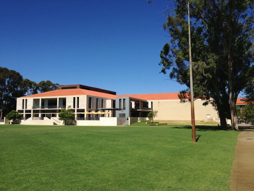
I have just got back from the 2013 Computer Applications in Archaeology (CAA) conference in Perth, Australia.  The conference was held in the University Club at the University of Western Australia:

UWA

UWA is in western Perth, close to the estuary of the aptly named Swan River:

Swan River

The conference overall was a fun one, with particularly interesting presentations by Oxford’s own John Pouncett and by his boyhood mentor, Dominic Powlesland.  I presented a paper in John and Gary Lock’s session on spatial scale, about how different scales inter-operate in the context of Englaid data.  I will summarise it on here at some point in the future, once we’ve thought through our ideas a bit more.

After the conference, I explored some distinctly non-English landscapes:

Pinnacles Desert

Moving on from my holiday snaps, I have been thinking a little more about temporal fuzziness with regards to PAS data (see previous post).  This time, I built in the data contained in the early medieval coin corpus at the Fitzwilliam Museum, Cambridge (EMC), to provide extra detail for the post-Roman period.

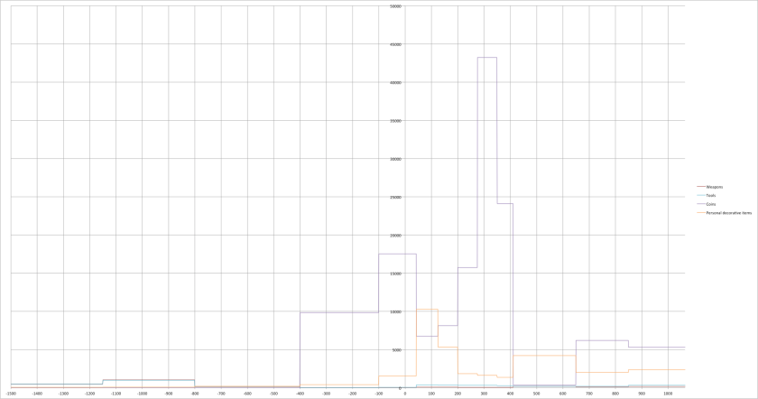
Using the “standard” time brackets discussed in the previous post, I then divided the data up according to (some of) our broad object type categories.  These are what we call “soft” categories, so that certain types of object can appear in more than one category (e.g. axes are categorised as both weapons and tools).  We can then produce graphs of the summed probabilities for each type, showing change in their deposition over time (x-axis is time, y-axis is summed probability):

PAS & EMC summed probability
Summed probability curves for combined PAS and EMC data, divided by broad type

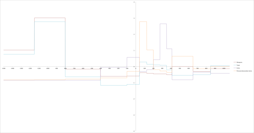
Obvious things to note are the peaks in coinage deposition in the late Iron Age and the 4th century and the peaks in personal decorative items in the early Roman and during the earliest early medieval.  However, because of the vastly different amounts of objects found in each category and in each time period bracket, it is hard to pick out subtler patterning.  To do so, we can calculate the mean value and standard deviation for each category and then express the values in variation from the mean (in standard deviations) for each category (x-axis is again time, y-axis is summed probability in plus or minus standard deviations [0 is the mean, +1 is +1 st. dev., -1 is -1 st. dev., etc.]):

PAS & EMC summed probability, stdev
Summed probability curves for combined PAS and EMC data, divided by broad type, plotted by standard deviations from mean value

This graph then shows the same patterns we could draw out from the previous graph, but brings out various other details.  Most obvious is the huge peak in weapons and tools in the Bronze Age (especially later), but other patterns also come out (relatively high amount of tools during the Roman period; relatively high amount of weapons [i.e. average] in the earliest early medieval; etc.).

Similar graphs could be produced for regions of the country, rather than types, or for types within a region of the country.  These ideas still need further exploration, but I think they begin to show the power of using a fuzzy probability approach to the analysis of the temporality of our data.

Chris Green